Blog post
When Does "Cloning" Work for Reject Inference?
Naftali Harris
Published
November 20, 2024

There's a big challenge in statistical credit models: you only get to see the performance of applicants to whom you gave a loan. Applicants that were rejected never had the opportunity to either pay you back or default, so you don't have any performance labels for them to use in modeling.
The most basic way to treat this is to restrict the training set to just applicants who actually received a loan, and fit a model to predict their repayment using characteristics known about them at the time of application (e.g. attributes from their credit report). But this biases the training set significantly compared to the actual distribution of applicants (in particular, the training set will be more creditworthy) and discards the real information about other applicants.
So credit modelers sometimes try to use "reject inference", which refers to a collection of methods of trying to incorporate data about the rejected population into their modeling. There are a lot of ideas here—one for example is to use credit bureau data to look at the credit performance of the rejected population with other financial products.
But perhaps the simplest method of reject inference is what's called "cloning". With cloning, you start by fitting a model on the approved population and using it to make predictions on the rejected population (the "reject inference model"). Then you take these predictions on the rejected population, treat them as targets, and refit the model on the entire population of applicants using the actual performance for the approved population and the inferred performance for the rejected population. The intuition here is that you're trying to figure out what the label would/should have been for the rejected population and then including that population in the final model.
Concretely, in a binary classification context, if the reject inference model predicted that a particular rejected applicant had a 70% chance of repayment, you would "clone" the rejected applicant into two separate observations. The first clone gets a "repay" label, and an observation weight of 0.7. The second clone gets a "default" label, and an observation weight of 0.3. Then you concatenate the "repay" and "default" clones to the approvals dataset, and fit your binary classifier on it.
Now if you're skeptical about this actually doing anything... you'd be at least partially right. For many configurations of this problem setup, the final model on both the approved and rejected populations will be literally identical to a model fit just on the approved population. Let's have a look:
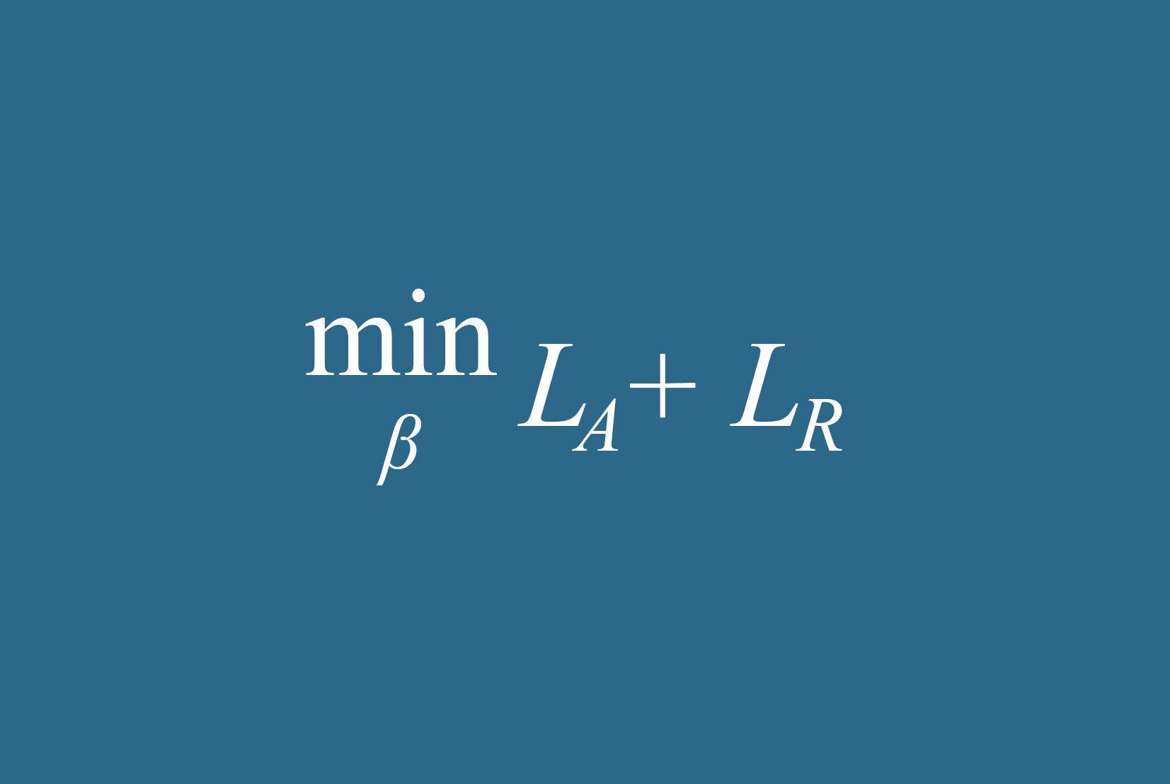
Most binary classifiers solve some kind of optimization problem to minimize the prediction error on the training data. Call the loss function for the approved dataset L_A, and the loss function on the cloned rejected dataset L_R. The model on approvals tries to minimize L_A, and the full model tries to minimize L_A + L_R.
Now, for any reasonable prediction-error based loss function you could pick (e.g. log likelihood), the prediction error for the reject sample will in fact be minimized at the original predictions. (The thing you're trying to predict was the inferred label, which is the original prediction itself—so go ahead and make the same prediction again). As a result, the original model on just the approvals also optimizes L_R.
Since the approvals model optimizes both L_A and also L_R, it minimizes their sum L_A + L_R, and therefore the approvals model will also end up being the full population model. And not approximately, exactly—the model on the full population will literally be the exact same model as the one fit only on approvals. (If you don't believe the math, see the numerical simulation in the gist at the end of this article).
So how does this break? At least two major ways:
Firstly, many optimization problems used in statistical machine learning are solved inexactly. The logic above works if you solve the optimization problem perfectly. In practice, the set of problems solved exactly tends to be the ones with convex loss functions, such as logistic regression. But non-convex optimization problems deriving from e.g. tree-based or neural-net based approaches are solved inexactly, and so these results no longer hold. I don't have a strong intuition for this, but arguably in this case the full model is learning at least something from the rejected population, specifically that the applicant population isn't just limited to approvals and that it should prioritize separation on the rejected population in addition to separation on the approved population.
Secondly, if you use a different type of model to infer labels for the rejected population than you do for the final model, you'll also obviously end up with a different model. The same is true if you use different features to do the label inference compared to the final model. For credit problems in particular, this may be especially relevant since there are legal, regulatory, and policy-based constraints on the model features and form of credit models, which may be looser for the reject inference model. In this case it's clear that the full model is actually learning from the rejected population, since it's being supplied new information from the looser reject inference model.
(Disclaimer: SentiLink provides identity fraud prevention services, not credit eligibility or assessment services. This is an article about statistics, theoretical machine learning, and numerical optimization, not legal requirements or regulatory policy. Please consult your own legal counsel and other advisors when building credit models.)
Related Content

Blog article
April 14, 2026
The Montana Loophole Is Closing. Are Lenders Holding the Bag?
Read article
Blog article
April 1, 2026
Inside "Pell Running," the Federal Student Aid Fraud Congress Is Trying to Stop
Read article
Blog article
March 30, 2026